July 2, 2020

By Danfoss Drives

The inverter is the last of the main elements making up the AC drive. The inverter processes represent the final stage in terms of generating the output voltage and frequency. When the motor is connected directly to the mains, the ideal operating conditions apply at the rated operating point.

The AC drive guarantees good operating conditions throughout the whole speed range by adapting the output voltage to the load conditions. It is thus possible to maintain the magnetization of the motor at the optimal value.

From the intermediate circuit, the inverter obtains one of the following:

– Variable direct current

– Variable DC voltage

– Constant DC voltage

In each case, the inverter must ensure that the supply to the motor is an AC voltage. In other words, the frequency of the motor voltage must be generated in the inverter. The inverter control method depends on whether it receives a variable or a constant value. With a variable current or voltage, the inverter only needs to generate the corresponding frequency. With a constant voltage, the inverter generates both the frequency and amplitude of the voltage.

Even though inverters work in different ways, the basic design is always the same. The main components are controlled semiconductors, arranged in pairs in three branches, as shown in

Transistors are increasingly taking the place of thyristors in the inverter stage of AC drives for several good reasons. Firstly, transistors are now available for large currents, high voltages and high switching frequencies. Furthermore, unlike thyristors and diodes, transistors are not affected by the current zero crossing. Transistors can enter the conducting or blocking state at any time simply by changing the polarity of the voltage applied to the control terminals. The advances made in the field of semiconductor technology over recent years have increased the switching frequency of transistors significantly. The upper switching limit is now several hundred kHz.

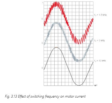Thus, magnetic interference caused by pulse magnetization within the motor can be avoided. Another advantage of the high switching frequency is the fact that it allows variable modulation of the AC drive output voltage. This means that a sinusoidal motor current can be achieved, as shown in Fig. 3.13 Effect of switching frequency on motor current. The control circuit of the AC drive merely has to switch the inverter transistors on and off in accordance with a suitable pattern.

The choice of the inverter switching frequency is a trade-off between losses in the motor (sine shape of motor current) and losses in the inverter. As the switching frequency increases, so do the losses in the inverter, in line with the number of semiconductor circuits.

High-frequency transistors can be divided into three main types:

– Bipolar (LTR)

– Unipolar (MOSFET)

– Insulated Gate Bipolar (IGBT)

Table 3.2 Comparison of power transistor characteristics shows the IGBT transistors are a good choice for AC drives in terms of the power range, the high level of conductivity, the high switching frequency and ease of control. They combine the features 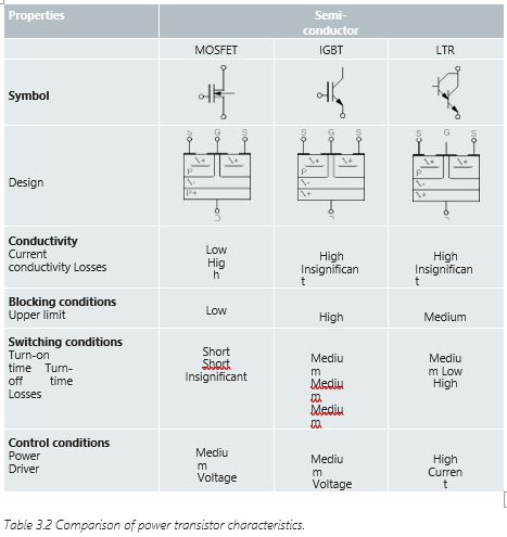of MOSFET transistors with the output properties of bipolar transistors. The actual switching components and inverter control are normally combined to create a single module called an “intelligent power module” (IPM).

A freewheeling diode is connected in parallel with each transistor, because high induced voltages can occur across the inductive output load. The diodes force the motor currents to continue flowing in their direction and protect the switching components against imposed voltages. The reactive power required by the motor is also handled by the freewheeling diodes.

key differences between MOSFET, IGBT and LTR transistors.

3.6 Modulation Principles

The semiconductors in the inverter either conduct or block according to the signals generated by the control circuit. The variable voltages and frequencies are generated using two basic principles (types of modulation):

– Pulse Amplitude Modulation (PAM) and

– Pulse Width Modulation (PWM)

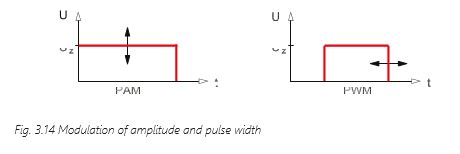
3.6.1. Pulse Amplitude Modulation (PAM)

PAM is used in AC drives with variable intermediate circuit voltage or current. In drives with uncontrolled or half-controlled rectifiers, the amplitude of the output voltage is generated by the intermediate circuit chopper, shown in Fig. 3.9 Variable DC voltage intermediate circuit. In a case where the rectifier is fully controlled, the amplitude is generated directly. This means that the output voltage for the motor is made available in the intermediate circuit.

The intervals during which the individual semiconductors should be on or off are stored in a pattern, and this pattern is read out at a rate dependent on the desired output frequency.

This semiconductor switching pattern is controlled by the magnitude of the intermediate circuit variable voltage or current. If a voltage-controlled oscillator is used, the frequency always follows the amplitude of the voltage.

Using PAM can result in lower motor noise and very minor efficiency advantages in special applications like high speed motors (10.000 – 100.000 RPM). However, this often does not overrule the drawbacks like higher costs for the more sophisticated hardware and control issues like higher torque ripples at low speed.

3.6.2 Pulse width Modulation (PWM)

PWM is used in AC drives with constant intermediate circuit voltage. This is the most widely- established and best developed method. Compared with PAM, the hardware requirements for this modulation method are lower, control performance at low speed is better and brake resistor operation is always possible.

The motor voltage can be varied by applying the intermediate circuit (DC) voltage to the motor windings for a certain length of time. The frequency can be varied by shifting the positive and negative voltage pulses for the two half periods along the time axis.

Because the technology varies the width of the voltage pulses, it is called ”Pulse Width Modulation” or PWM. With conventional PWM techniques, the control circuit determines the on and off times of the semiconductors in a way which 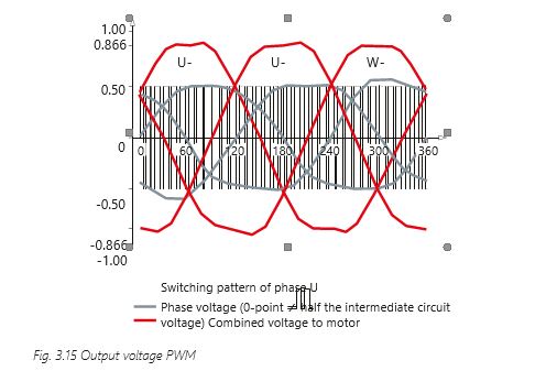makes the motor voltage waveform as sinusoidal as possible. Thus, the losses in the motor winding can be reduced and a smooth motor operation, even at low speed is achieved.

The output frequency is varied by connecting the motor to half the intermediate circuit voltage for a specific period of time. The output voltage is varied by dividing the voltage pulses of the AC drive output terminals into a series of narrower individual pulses with pauses in between.

The pulse-to-pause ratio can be modified depending on the required voltage level. This means that the amplitude of the negative and positive voltage pulses always corresponds to half the intermediate circuit voltage.

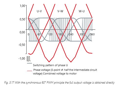
A low switching frequency leads to an increase in acoustic motor noise. To limit the amount of noise produced, the switching frequency can be increased. This has been made possible thanks to advances in the field of semiconductor technology, which mean that the generation of an approximately sinusoidal current is now achievable. A PWM AC drive that relies exclusively on sinusoidal reference modulation can provide up to 86.6% of the rated voltage (see Fig. 3.15 Output voltage PWM).

The phase voltage at the AC drive output terminals corresponds to half the intermediate circuit voltage divided by Ö2 and is thus equal to half the mains line voltage. The line voltage of the output terminals is equal to Ö3 times the phase voltage and is thus equal to 0.866 times the mains supply voltage.

The output voltage of the AC drive cannot equal the motor voltage if full sinusoidal wave form is needed, as the output voltage would be roughly 13 % too low. However, the extra voltage needed can be obtained by reducing the number of pulses when the frequency exceeds approximately 45 Hz. The disadvantage of using this method is that it makes the voltage

alternate step-wise and the motor current becomes unstable. If the number of pulses is reduced, the harmonic content at the AC drive output increases. This results in higher losses in the motor.

For example, one common reference voltage uses the third harmonic of the sine reference.

By increasing the amplitude of the sine reference by 15.5 % and adding the third harmonic, a switching pattern for the inverter semiconductors can be obtained which increases the output voltage of the AC drive. All control values of the inverter are transmitted from the control board, and the various reference signals for determining the switching times are stored in a table in memory and are then read out and processed according to the reference value.

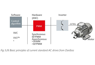
There are other ways of determining and optimizing the on and off switching times of the semiconductors. The Danfoss VVC and VVC+ control principles are based on microprocessor calculations which identify the optimum switching times for the inverter semiconductors (see chapter 2.8).

The specifications for the software involved in calculating the switching times are manufacturer- specific and will not be covered here.

If more stringent requirements are imposed on the AC drive speed setting range and smooth- running characteristics, then the PWM switching times need to be determined by an additional digital IC rather than the microprocessor. For example, a DSP (Digital Signal Processor) or a FPGA (Field Programmable Gate Array) can determine the PWM switching times. This component incorporates the manufacturer’s proven knowledge. Meanwhile, the microprocessors are responsible for handling other control tasks.

– Asynchronous PWM

Two asynchronous PWM methods are described below:

– SFAVM (Stator Flux-oriented Asynchronous Vector Modulation)

– 60° AVM (Asynchronous Vector Modulation)

These enable the amplitude and angle of the inverter voltage to be changed in steps.

3.6.3.1 SFAVM

Stator Flux-oriented Asynchronous Vector Modulation (SFAVM) is a space-vector modulation method that makes it possible to change the inverter voltage arbitrarily, but step-wise within the switching time (in other words, asynchronously). The main purpose of this type of modulation is to maintain the stator flux at the optimum level throughout the stator voltage range, ensuring no torque ripple. Compared with the mains supply, a “standard” PWM supply will result in deviations in the stator flux vector amplitude and the flux angle. These deviations will affect the rotating field (torque) in the motor air gap and will cause torque ripple. The effect produced

by the deviation in amplitude is negligible and can be reduced by increasing the switching frequency.

The deviation in the angle depends on the switching sequence and can result in higher levels of torque ripple. Consequently, the switching sequence must be calculated in such a way as to minimize the deviation in the vector angle.

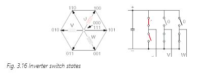
Each inverter branch of a 3-phase PWM inverter can assume two switch states, ON or OFF, as shown in Fig. 3.16 Inverter switch states. The three switches result in eight possible switch

combinations, leading in turn to eight discrete voltage vectors at the inverter output or at the stator winding of the connected motor. As shown below, these vectors (100, 110, 010, 011, 001,

101) mark the corners of a hexagon, where 000 and 111 are zero vectors.

With switch combinations 000 and 111, the same potential occurs at all three output terminals of the inverter. This will be either the positive or negative potential from the intermediate circuit, as shown in Fig. 3.16 Inverter switch states. As far as the motor is concerned, this is the equivalent to a terminal short circuit and so a voltage of 0 V is applied to the motor windings.

Generation of motor voltage

Steady-state operation involves controlling the machine voltage vector Uωt on a circular path. The length of the voltage vector is a measure of the value of the motor voltage and the speed of rotation corresponds to the operating frequency at a specific time. The motor voltage is generated by briefly pulsing adjacent vectors to produce an average value.

Some of the features of the Danfoss SFAVM method are as follows:

– The amplitude and angle of the voltage vector can be controlled in relation to the preset reference without deviations occurring

– The starting point for a switching sequence is always 000 or 111. This enables each voltage vector generated to have three switch states

– The voltage vector is averaged by means of short pulses on adjacent vectors as well as the zero vectors 000 and 111

SFAVM provides a link between the control system and the power circuit of the inverter. The modulation is synchronous to the control frequency of the controller and asynchronous to the fundamental frequency of the motor voltage. Synchronization between control and modulation is an advantage for high- power control (for example, voltage vector, or flux vector control), since the control system can control the voltage vector directly and without limitations. Amplitude, angle and angular speed are controllable.

In order to dramatically reduce the real-time calculation time, the voltage values for different angles are listed in a table. Fig. 3.18 Output voltage (motor) – (phase-phase) shows the motor voltage at full speed.

Low Speed Performance

Continuously pulsing all six inverter IGBTs to simulate the required output sine wave is ideal for low speed operation. It ensures smooth motor operation and allows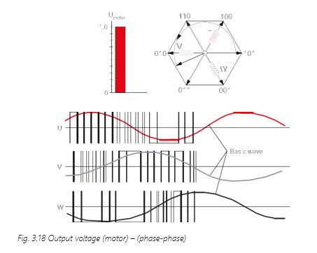 the drive to meet the demanding requirements of starting high friction or high inertia loads. However, this switching pattern is not suited for high speed operation. Continuously pulsing all six inverter IGTBs causes extra inverter switching losses, increased heat generation, and reduced drive efficiency. In addition, if a pure sine wave template is followed for each line-to-neutral voltage, the maximum output voltage is limited to 87% of the input voltage. This makes it impossible to produce rated motor power without exceeding rated motor current. To obtain higher full speed voltages, some conventional PWM drives add third and ninth harmonics to their reference AC wave. Without full voltage on the motor, conventional PWM waveforms use the motor’s service factor to produce rated output from the motor. This reduces motor life.

– 60° AVM

If 60° AVM (Asynchronous Vector Modulation) is used – as opposed to the SFAVM principle – the voltage vectors are determined as follows:

– Within one switching period, only one zero vector (000 or 111) is used

– A zero vector (000 or 111) is not always used as the starting point for a switching sequence

– One phase of the inverter is held constant for 1/6 of the period (60°). The switch state (0 or 1) remains the same during this interval. In the two other phases, switching is performed in the normal way

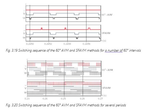Fig. 3.19 Switching sequence of the 60° AVM and SFAVM methods for a number of 60° intervals and Fig. 3.20 Switching sequence of the 60° AVM and SFAVM methods for several periods compare the switching sequence of the 60° AVM method with that of the SFAVM method – for a short interval (Fig. 3.19) and for several periods (Fig. 3.20).

High Speed Efficiency and Full Motor Output

Because of the high-speed limitations of SFAVM, the 60° AVM is preferred above a predefined output frequency. Above this speed, the microprocessor control holds each IGBT on for 60° of the full cycle and off for another 60° of the full cycle. By doing no switching in each inverter IGBT during 120° of each output cycle, the drive minimizes switching losses. In addition, this unique switching pattern allows the drive to provide the motor with full rated voltage. This allows the motor to produce full rated torque at full speed without creating excessive motor heating.

3.7 Control Circuit and Methods

The control circuit, or control board, is the fourth main component of the AC drive. The three hardware components dealt with so far (rectifier, intermediate circuit and inverter) are nearly always based on the same principles and components regardless of the manufacturer. In most cases, these components are standard, nearly always purchased from the same external manufacturers. The control circuit design stands in contrast to these, as the area where the AC drive manufacturer concentrates all its acquired knowledge.

In principle, the control circuit has four main tasks:

– Controlling the AC drive semiconductors. The semiconductors determine the anticipated dynamic characteristics or accuracy

– Exchanging data between the AC drive and peripherals (PLCs, encoders)

– Measuring, detecting and displaying faults, conditions and warnings

– Performing protective functions for the AC drive and motor

Using microprocessor technology, with single or dual processors, it is possible to increase control circuit speeds using ready-made pulse patterns that are stored in memory. As a result, there is a significant reduction in the number of calculations required.

With this type of control, the processor is integrated into the AC drive and is always able to determine the optimum pulse pattern for each operating stage. There are a variety of control methods available for determining the dynamic characteristics and response time in the event of a change in reference or torque as well as the positioning accuracy of the motor shaft.

In general, the basic functions of an AC drive can be summed up as follows:

Rotating and positioning the rotor
Open or closed-loop speed control of the AC motor
Open or closed-loop torque control of the AC motor
Monitoring and signaling operating states

Categorizing the various voltage-source AC drives available on the market (according to the form of control), at least six different types can be identified:

Simple (scalar) without compensation control
Scalar with compensation control
Space vector control
Open loop flux (field-oriented) control
Closed loop flux (field-oriented) control
Servo-controlled systems

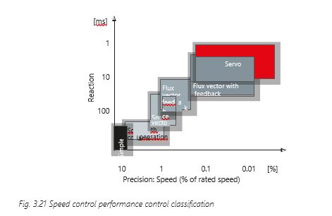This classification is illustrated in Fig. 3.21 Speed control performance control classification and Fig. 3.22 Torque performance control classification. Here, the reaction time refers to how long the AC drive needs to calculate a corresponding signal change to its output when there is a signal change at the input. The motor characteristics determine how long it takes to register a response on the motor shaft when an input signal is applied to the input of the AC drive.

The rated motor frequency is used as the basis for establishing the speed accuracy. The rated motor frequency is 50 Hz in most countries, and 60 Hz in the US. AC 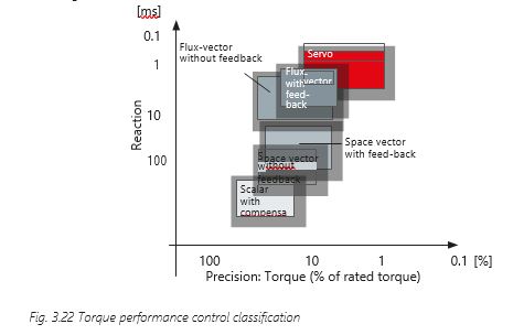drives can be classified according to price/performance ratio. That is, an AC drive that uses a simple control method is better value for money for performing very simple tasks, than one featuring field-oriented control.

The speed setting ranges associated with the individual AC drive types are roughly as follows:

Simple (scalar) without compensation 1:15
Scalar with compensation 1:25
Space vector 1:100(0)
Flux (field-oriented) open loop 1:1000
Flux (field-oriented) close loop 1:10.000
Servo 1:10.000

The torque control performance can be classified as follows:

The reaction time may be defined in the same way as for speed control
The accuracy is determined in relation to the motor’s rated torque

Please note that AC drives that rely on a simple control method cannot be used for either open- loop or closed-loop control of the motor torque.

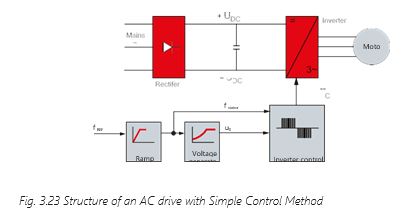
Simple control method

This type of control is rarely used today. The control is in principle a fixed relationship between desired motor speed and a motor voltage. The model can be more or less refined, but the major disadvantages are:

Unstable motor speed
Difficult start of the motor
No protection of the motor

The only advantage of simple control could be the low price, but since basic components for sensing motor characteristics are relatively low-cost, very few manufacturers now pursue this method.

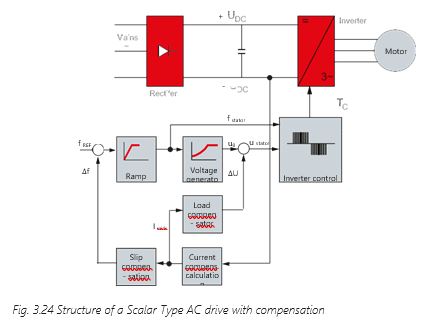
When compared with simple control, an AC drive with compensations adds three new control function blocks as illustrated in Fig. 3.24 Structure of a Scalar Type AC drive with compensation.

The load compensator uses the current measurement to calculate the additional voltage (ΔU) required to compensate for the load on the motor shaft.

The current is typically measured by means of a resistor (shunt) in the intermediate circuit. It is assumed that the power in the intermediate circuit is equal to the power consumed by the motor. If several active switch positions are combined, these can be used to reconstruct all the phase current information.

Basic features:

Voltage/frequency [U/f ] control with load and slip compensation
Control of voltage amplitude and frequency

Typical shaft output:

Speed setting range 1:25
Speed accuracy ±1% of rated frequency
Acceleration torque 40-90% of rated torque
Speed change response time 200-500 ms
Torque control response time Not available

Typical features:

Improved control properties compared with simple scalar control
Able to withstand sudden changes in load
No external feedback signal required
Unable to solve resonance problems
No torque control properties
Problems occur when attempting to control high-power motors
Problems in the event of load changes in the low speed range

Space Vector with and without Feedback

The space vector control method is available with (“closed loop”) or without (“open loop”) an external motor speed feedback. A feature allowing motor current polar transformation is

added to the control (in the components responsible for magnetization and torque-generating current).

The voltage angle (θ) is regulated in addition to the voltage (U) and frequency (f ).

Basic features:

Voltage vector control in relation to steady-state characteristic values (static)

Typical features:

Improved dynamic performance compared with scalar control
Very good at withstanding sudden changes in load (compared with scalar plus compensation)
Operation at the current limit
Possibility of active resonance dampening
Possibility of open-loop/closed-loop torque control
High starting and holding torque
Problems during rapid reversing compared with flux vector
No “rapid” current control

Space Vector (Open Loop)

If the space vector is determined without external speed feedback then the speed and position will be calculated by the control software and is based on information about motor current and motor frequency which is measured (see example on page 77, Fig. 3.28 Basic principles of Danfoss VVC+ control).

Basic features:

Voltage vector control in relation to steady-state characteristic values (static)

Typical shaft output:

Speed setting range 1:100
Speed accuracy (steady state) ± 0.5% of rated frequency
Acceleration torque 80-130% of rated torque
Speed change response time 50-300 ms
Torque change response time 20-50 ms

Space Vector (Closed Loop)

For the closed loop space vector method, an encoder or other device to detect the motor speed or position is required. It is the control software, the resolution on the feedback input and encoder’s resolution that determines the accuracy of motor control.

Typical shaft output:

Speed setting range 1:1000 – 10000
Speed accuracy (steady state) Depends on resolution of feedback component used
Acceleration torque 80 – 130% of rated torque
Speed change response time 50 – 300 ms
Torque change response time 20 – 50 ms

Open Loop and Closed Loop Flux Vector Control

Flux vector control is also referred to as field-oriented control. The control methods referred to above control the motor magnetic flux via the stator. With field-oriented control, the rotor flux is controlled directly. The following motor variables are controlled within this context:

Speed
Torque

Once the rated data for the motor has been entered, a magnetic flux model can be used to determine the necessary voltage and angle for ensuring optimum motor magnetization. The measured motor current is converted into a torque-generating current and a magnetizing current. An internal PID controller is responsible for controlling the speed, with the feedback value being estimated on the basis of the measured motor current.

Flux Vector (Open loop)

Flux control requires accurate information about the condition, temperature and rotor position of the motor. It is a challenge to run open loop while the motor condition is being simulated. Obtaining optimum performance can be difficult, especially at low motor speed.

Typical shaft output:

Speed setting range 1:1000
Speed accuracy (steady state) ± 0.5% of rated frequency
Acceleration torque 100-150% of rated torque
Speed change response time 50-200 ms
Torque change response time 5-5 ms

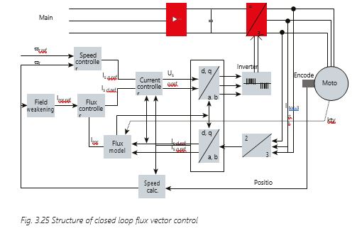
Flux Vector (Closed Loop)

For the closed loop flux vector control method, an encoder or similar sensor is required on the motor shaft. The control software and the feedback resolution determine the accuracy of motor control.

Control is performed in exactly the same way as with open loop methods. However, in this case the speed is calculated from the encoder signals rather than being estimated. Flux vector control is illustrated in Fig. 3.25 Structure of closed loop flux vector control.

Typical shaft output:

Speed setting range 1:1000 – 10000
Speed accuracy (steady state) Dependent on the feedback signal (encoder) used
Acceleration torque 100 – 150% of rated torque
Speed control response time 00 – 50 ms
Torque control response time 50 – 5 ms

3.7.5 Servo Drive Control

The servo converter control method will not be explored in depth here. One common method is very similar to closed loop flux control, but to ensure high dynamic response, the power components and hardware may be upgraded as much as two, three or four times the power components in an AC drive to ensure available current and torque.

Integrated Motion Controller

Positioning and synchronization operations are typically performed using a servo drive or a motion controller. However, many of these applications do not actually require the dynamic performance available from a servo drive.

High-precision positioning and synchronization can also be performed simply using an AC drive. To save time and cost, Danfoss has developed the Integrated Motion Controller (IMC) functionality, which can replace more complex positioning and synchronization controllers in single-axis positioning and synchronizing applications.

The IMC can be set to run in Positioning, Synchronizing or Homing mode.

Positioning

In positioning mode, the drive controls movement over a specific distance (relative positioning) or to a specific target (absolute positioning). The drive calculates the motion profile based on target position, speed reference and ramp settings. There are 3 positioning types using different references for defining the target position:

Absolute positioning: Target position is relative to the defined zero point of the machine
Relative positioning: Target position is relative to the actual position of the machine
Touch probe positioning: Target position is relative to a signal on a digital input

Synchronizing

In synchronizing mode, the drive follows the position of a master. Multiple drives can follow the same master. The master signal can be an external signal e.g. from an encoder, a virtual master signal generated by a drive or master positions transferred by fieldbus. Gear ratio and position offset is adjustable by parameter.

Homing

With sensorless control and closed loop control with an incremental encoder homing is required to create a reference for the physical position of the machine after power up. There are several home functions with and without sensor to choose from. The home synchronizing function can be used to continuously realign the home position during operation when there is some sort of slip in the system. For example, in case of sensorless control with an induction motor or in case of slip in the mechanical transmission.

In conclusion, all control methods are primarily handled by the software. The more dynamic the motor control needs to be, the more complex the control algorithm required.

A similar principle applies for initial use of an AC drive. Initial use of a simple AC drive does not involve a great deal of programming. In most cases, all you have to do is enter the motor data. However, for applications that require a flux vector control or critical applications like hoists, more complex programming is required, right from initial use.

Because the control is mainly a software issue, many manufacturers have implemented several control methods in their units, for example U/f, space vector, or field-oriented control.

Parameters are needed to switch from one control method to another, for example from space vector control to the flux vector method. Pop-up menus help the operator to set the parameters needed for each control method, in order to meet the application demands.

Chapter 3, Sections 3.1 – 3.5

Chapter 3, Sections 3.8 – 3.9.2